
Chapter 7 Similiters and Suchness
The ‘suchness’ or quality of homeopathy is continually being discussed or challenged. In the “Organon of Medicine” [1] , Hahnemann wrote in #22, “…that for the totality of symptoms to be cured, one must seek that medicine which has demonstrated the greatest propensity to produce either similar or opposite symptoms”.
This Chapter will build on what has been discussed in previous Chapters. In particular, that the language of bio-communication and homeopathy is expressed as patterns of frequencies and phases. This leads to the idea that frequencies indicate stress in patients. Endogenous frequencies on acupuncture meridians and characteristic frequencies in chemicals interacting with water (bulk or trace) are developed into homeopathic potencies by serial dilution and succussion. Importantly, Hahnemann noticed that the effects of his medicines were ‘bi-phasic’ in that they produced either similar or opposite symptoms, patterns of frequencies show this effect and become a cure for Hahnemann’s totality of symptoms.
Two important theoretical and mathematical concepts will be introduced, Fractals and Chaos. The essential characteristic of a Fractal is self-similarity. Chaos is random behaviour in a system operating according to scientific laws and equations. If living systems can become chaotic, the minimals of a homeopathic potency can lead to a major therapeutic effect. There is a so-called “butterfly effect” whereby, at least in the mathematical theory of weather systems, a butterfly flapping its wings in the Amazon can trigger a hurricane in the Caribbean.
7.1 Fractality of Frequencies
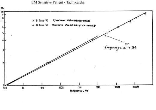
There is self-similarity in the symptoms triggered in electromagnetically hypersensitive patients by different frequencies. Figure 1 is an example in which a patient whose tachycardia was triggered by the electrical environment. On 5 June 1990, the frequencies giving neutralisation were assessed by clinical observation but this was a slow process and the testing had to be halted when the pulse rate went too high. On the 19 June 1990, the patient was assessed by observation of a pulse-rate meter and the frequency adjusted to get pulse rates as near normal as possible. This set of measurements was in good agreement with those made a fortnight earlier. The technique was objective which is a rare possibility in this work and allowed nine harmonics to be measured. This patient’s neutralising frequencies f are given by the following empirical equation where n is the number of the harmonic:
f = n7.7 +126 Hz

Figure 1
Each point shows a frequency at which the pulse rate increases triggered by the remaining frequencies was neutralised.
This type of fractal behaviour is characteristic of the provocation and neutralisation of allergic and hypersensitivity reactions by the “Miller Technique” (see Section 2.8).
In Section 3.4, it was shown that the equation determining the frequency imprint depends on the dilution ratio used and the number of potentisations N.
Dilution ratios of 100 (C potencies) are unusual in that the equation is linear in potency although logarithmic in concentration:
( f / f0 ) = N ( dilution ratio = 100 ).
f n+1 = f n ( dilution ratio = 100 )N
The results for the remaining dilution ratios tested are best plotted on a log/log scale but they do not give straight line plots. They can be approximated by straight line sections and in general, are represented by the equation:
log f/f0 = N r log(dilution ratio)
where N = the serial number of the dilution (or the potency). The means and standard deviations for r are given in Table 1 for different dilution ratios.
Table 1
Experimental Values of r for Different Dilution Ratios for the first 10 Potentisations
|
Dilution Ratio |
r |
|
2-Fold |
1 |
|
3-Fold |
1 |
|
4-Fold |
0.561 ± 0.040 |
|
5-Fold |
0.411 ± 0.083 |
|
10-Fold |
0.551 ± 0.029 |
|
1000-Fold |
0.098 ± 0.004 |
Before dilutions reach Avogadro’s Number, the curve has had a change of slope as shown in Figure 3 of Section 3.3. The equation then is:
log ( f / f0 )= r N (log 10)
where at potencies < 6, r = 0.35 and at potencies > 6, r = 0.11. These figures come from approximate fit to the curve.
A slope change is also characteristic of the frequency pattern set up as a result of decimal potentisation of thyroxin (see Section 3.2). In this case, the frequency f is given by the equation:
log ( f / f0 )= r N (log 10)
where f0 is a frequency of the “Mother Tincture”; for N < 18, r = 0.5 and for potencies N > 18, r = 0.16.
All these equations could be descriptions of fractal systems. In Table 1 of Section 4.2, the pattern of frequencies in water which had been imprinted with the optical spectrum of mercury vapour have a fractal similarity at microwaves and at low frequencies with standard deviations less than 1%. Examples of fractal similarity at different frequencies have already been presented are summarised in the following Table 2.
Table 2
Examples of the Fractality of Frequencies presented in Previous Sections.
| Section |
Table |
|
|
2.9 |
3 |
Frequencies Endogenous to Acupuncture Meridians |
|
2.10 |
4 |
Frequency Entrainment at Acupuncture Point |
|
3.6 |
2 |
FIR and ELF Resonances in n-Hexane |
|
4.2 |
1 |
Mercury Spectrum Imprinted in Water |
|
5.11 |
2 |
Modelling Hexane and Water Molecules |
7.2 More on Fractality
Any effect which involves an oscillation of frequency f and wavelength ? propagating with velocity v has these three quantities related by the equation:
f × ? = v
However within a coherent system, the coherence length replaces the wavelength and becomes the constant quantity. This makes the velocity proportional to frequency.
This consequence of coherence has forced itself on my awareness many times. It makes frequency a fractal quantity with no absolute scale of magnitude. Any velocity that the system can support will have a corresponding and proportionate frequency. Each frequency can and will interact with the others. It is this which links the spectra of chemical reactions to the technological and biological frequencies.
In such a system, external radiation will only interact with an entire coherence domain. Because of its large mass, the velocity is decreased from the velocity of light (3×10⁸ m/s) to something of the order of metres per second. Thus, one finds at least two fractal frequencies, one corresponding to the velocity of coherence the other to the velocity of light.
Measurements were made of the velocity with which coherence propagates by measuring the time taken to cover a known distance using a transistor (FET) at each end of the specimen to interrupt the propagation of the coherence. Additionally, measurements of the critical angle at an air interface gave similar velocities. The measured velocity for coherence in water was 2.6 m/s and the velocity measured along a leg was 6 m/s. Comparison of these high-to-low frequency ratios for several systems is given in Table 3 where:
- Row 1gives the ratio of the FIR spectra frequencies for the n-alkanes to measured ELF resonances.
- Row 2 The crucial question here was whether the same argument could be applied to the interaction between water laser lines in the absence of an n-alkane. The ratios for the FIR water lines and measured water resonances in the GHz and ELF given in this row show that this is a possibility. If for the GHz/ELF ratio the GHz velocity is taken as 3×10⁸ m/s, the ELF velocity becomes 2.875 m/s (SD ±3.4%) and compares with the 2.6 m/s measured for water.
- Rows 3 & 4 give the frequency ratios for the spectrum from a mercury lamp imprinted into water showing a two stages of fractality.
- Row 5 compares the fractal ratios for water imprinted with frequencies between 1 mHz – 10 mHz and measured between 200 MHz – 2 GHz with the converse.
- Rows 6-11relate to measurements on the chakra points and the acupuncture meridians in humans. The frequency 384 MHz is the high band frequency of the heart acupuncture meridian and chakra, its lower frequency is 7.8 Hz corresponding to a coherence propagation velocity of 6.1 m/s compared with the 6 m/s measured in a human leg.
Table 3
Frequency Ratios – velocity of light to velocity of coherence
|
System |
Mean Ratio |
Standard Deviation |
|
|
1 |
n-alkanes with trace waterFIR(tables)/ELF(measured) |
1.97×10¹¹ |
±8% |
|
2 |
Water laser lines FIR/GHzGHz / ELF |
1.722×10³ 1.085×10⁸ |
±2.4% ±4.6% |
|
3 |
Mercury spectrum in wateroptical/microwave |
1.734×10⁶ |
±0.34% |
|
4 |
Mercury spectrum in watermicrowave/ELF |
47.70×10⁶ |
±0.75% |
|
5 |
Water imprinted ELF measured microwaveWater imprinted microwave measured ELF |
1.98×10¹¹ 2.09×10¹¹ |
±3.5% ±20% |
|
6 |
Chakra points |
48.76×10⁶ |
±1.5% |
|
7 |
Acupuncture meridians(mean stimulating frequencies) |
49.19×10⁶ |
±0.15% |
|
8 |
Acupuncture meridians(mean endogenous frequencies) |
48.61×10⁶ |
±3.0% |
|
9 |
Acupuncture meridians (subject #1)(subject #2) |
48.54×10⁶ 47.22×10⁶ |
±3.0% ±6.9% |
|
10 |
Microscope slides of target organ specimens |
50.97×10⁶ |
±12% |
|
11 |
Heart Meridian entrained to microwaves270-480 MHz / 5.2-7.6 Hz |
50.80×10⁶ |
±9% |
Coherence can propagate with superluminal velocity if the imprinted frequency is appropriate. Energy is only involved in the initial setting up of the coherence domains.
This velocity can be detected between living systems and also for water imprinted at a frequency higher than a natural resonance corresponding to the velocity of light. It is measured using the critical angle for total internal reflection at an air-water interface. For superluminal velocities the critical angle appears on the air side of an air/water interface and not in the water.
Figure 2 shows this effect for a pair of earthworms with their endogenous frequencies synchronised. Work in cooperation with Dr. Christian Endler in Graz showed that tadpoles could have their endogenous frequencies synchronised and that this synchronism was retained so long as they were in optical contact in the yellow or shorter wavelengths [2] (Afterwards, the earthworms returned to feed happily in the compost bin). If coherence in living systems enables them to communicate superluminally, they have the Maxwell Demon Effect available to them.
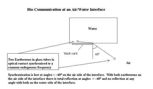
Figure 2
Superluminal Biocommunication between Synchronised Earthworms
7.3 Chaos
Chaos is something which occurs only in non-linear systems. While still functioning under precise control and according to recognised scientific laws, they may show unpredictable random-like behaviour under certain conditions. The outcome from any identical set of initial conditions is not repeatable but, it is not a truly random (stochastic) effect. Chaotic systems may show fractal properties like those just described.
Chaos cannot happen in the linear systems which are those favoured for mathematical analysis because the equations can be solved analytically. Linear systems are predictable but they are rare in Nature which is not deterministic although experimental conditions may be chosen so that linearity is approximated to.
Stewart [3] has written a very readable and non-mathematical account of the historical development of the concepts of chaos and its universality in the phenomena of science. Its title is Einstein’s famous question. A useful and not too mathematical text on fractals and chaos is a book by Addison [4] .
Chaos theory developed during Froehlich’s working career. He preferred pencil and paper and did not personally become involved in computing which is essential for the examination of equations which cannot be solve analytically. In his second “Green-Book” [5] his discussion of periodic enzyme reactions concludes with the equation of a limit cycle. He notes its oscillations are able to store energy, have stability against certain perturbations yet, a relatively small but appropriate perturbation may cause their collapse and the liberation of the stored energy. Chaos has been found experimentally by Olsen and Degn [6] in an enzyme reaction, the peroxidise catalysed oxidation of NADH in a system open to oxygen.
Froehlich leaves the computing to Kaiser [7] in the following Chapter who deals generally with the theory of non-linear excitations and points out that chaotic states must be viewed as an essential functional component of active biological systems parts of which may be in a chaotic state or can be driven into a chaotic one by external stimuli.
Femat (et al.) [8] studied the complete time series of heart signals obtained with an electrocardiogram. They found an oscillatory pattern involving signals arising from at least three frequencies associated with breathing, blood pressure and heart. Data analysis provided evidence for chaotic behaviour. Their results support the counterintuitive idea that in some biomedical systems, chaotic dynamical behaviour is normal. They also cite work on heart rate variability analysis which found that the interval fluctuates in a complex and apparently erratic manner even in healthy resting subjects.
Heart Rate Variability Analysis (Section 6.3) can be used to assess the status of the parasympathetic autonomic nervous system which in turn is related to Voll’s summation points on acupuncture meridians and these in turn can be stimulated with homeopathic potencies as discussed in Section 2.11. If the parasympathetic can have chaotic properties, why not the sympathetic ANS?
Section 2.4 covered the ‘Dallas Electrical Sensitivity Trials’ which were designed to demonstrate the reality of electrical sensitivities. These are a model of how to conduct such investigations. They were conducted in four phases:
- Development of a controlled test environment and test procedure.
- Single-Blind screening at frequencies 100 mHz – 5 MHz on 100 patients.
- Double-Blind tests on the 25 patients showing no reactions during placebos and 25 control patients.
- Two Double-Blind tests on 16 patients at their most sensitive frequency using 5 placebos to 1 active test.
In Phase 4, the 16 patients from Phase 3 who were twice re-challenged double-blind at each patient’s most sensitive frequency 100% reactions to the double-blind challenges, 0% reactions to the placebos each time. With such results where is there space for statistics? Yet, NIOSH dismissed these trials with the comment that since they had started with 100 subjects and only found 16 who were electrically sensitive, the results were not statistically significant.
The Dallas Trial results might be interpreted as follows. The 16 Phase 4 patients represent persons who were stable in a condition of disease and responded to testing in a linear manner always giving the same reactions to the same stimulus since double-blind testing did work for them.
Persons in a stable healthy state respond to testing in a linear manner and always give the same reactions to the same stimulus. Here, ‘Healthy’ means no hypersensitivity to the electrical environment. These would be the 25 patients in Phase 2 who gave 0% responses (EMF insensitive) and the Phase 3 and Phase 4 “Controls”.
The false positive patients (30 from Phase 2 and 2 from Phase 3) may have been in some chaotic state between health and disease. If correct, the implication is that homeopathy switches patients who are in some chaotic state between health and disease back to health. Because it is dealing with a chaotic condition it is fundamentally impossible to get the same response to the same stimulus each time homeopathy is used on these patients – therefore it is fundamental that homeopathy cannot be double-blind tested using these patients.
Some other way must be found to validate the effectiveness of homeopathy. It might be possible to use heart-rate variability to pre-test all trial patients to confirm that they are not in such a chaotic state but remembering the indications that some degree of chaos appears to be normal in any living system.
7.4 Similar and Opposite Symptoms
This Section returns to Hahnemann’s quotation above, “…one must seek that medicine which has demonstrated the greatest propensity to produce either similar or opposite symptoms”. All frequencies seem to have biphasic effects including frequency patterns in homeopathic potencies.
It has been one of the themes of these Chapters that homeopathic potencies contain patterns of frequencies which are the basis of their therapeutic effectiveness. Frequencies in the environment (Section 2.10 Table 4), frequencies imprinted into water or, the frequency signature of a chemical (Section 3.6 Table 1) can entrain acupuncture meridians whose endogenous frequencies happen to be nearby. Exceptionally, the Du Mai (Governing Vessel) meridian will become entrained to the strongest signal present at almost any frequency. Frequency entrainment is an essential characteristic of non-linear systems.
The frequencies characteristic of biological systems fluctuate by a small amount around their nominal value in a quasi-periodic manner, which may be chaotic. This applies to single cells as well as to the human system. An entraining frequency may accelerate this fluctuation or it may stop it altogether as seen in Figures 2 to 5. Thus, the frequency pattern of a homeopathic potency may stimulate or depress biological activity and it should be no surprise that the same potency can be “therapeutic” in the case of a patient who needs its particular frequency and phase but, “proving” in a healthy subject who needs no therapy.
Figure 2
Acetabularia – Frequency Fluctuation over 50 minutes
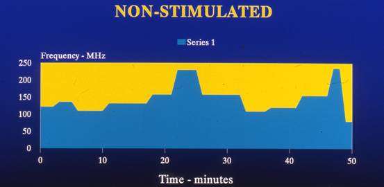
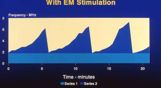
Figure 3
Acetabularia
Series 1 – Fluctuations cease under a depressive phase frequency.
Series 2 – Fluctuations speeded up under stimulatory phase frequency.
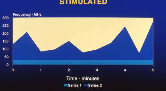
Figure 4
Human – Fluctuations of whole body frequencies over 2 hour period.
Fluctuations are not synchronised between the series of frequency bands.
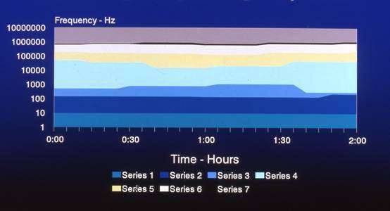
Figure 5
Human
Series 1 – Fluctuations cease under a depressive phase frequency.
Series 2 – Fluctuations speeded up under stimulatory phase frequency.
7.4 Similiters
In one case, involving an electrically hypersensitive patient, the frequencies of a homoeopathic potency already prescribed were exactly the frequencies found independently which the patient needed to have stimulated. In this case, the patient needed stimulation at: 1.5 Hz, 5.6 Hz and 1.6 kHz. The homeopathic potency Calcarea carb. 10M had been prescribed by a homoeopath. Measurements on a number of potencies of Calcarea carbonica showed that only the 10M potency of Calcarea carb. contained exactly these frequencies.
The common remedy Arnica has been described as the best traumatic. It has the frequency pattern given in Table 4. The acupuncture meridians influenced reflect the homeopathic effects for which it might be a similiter.